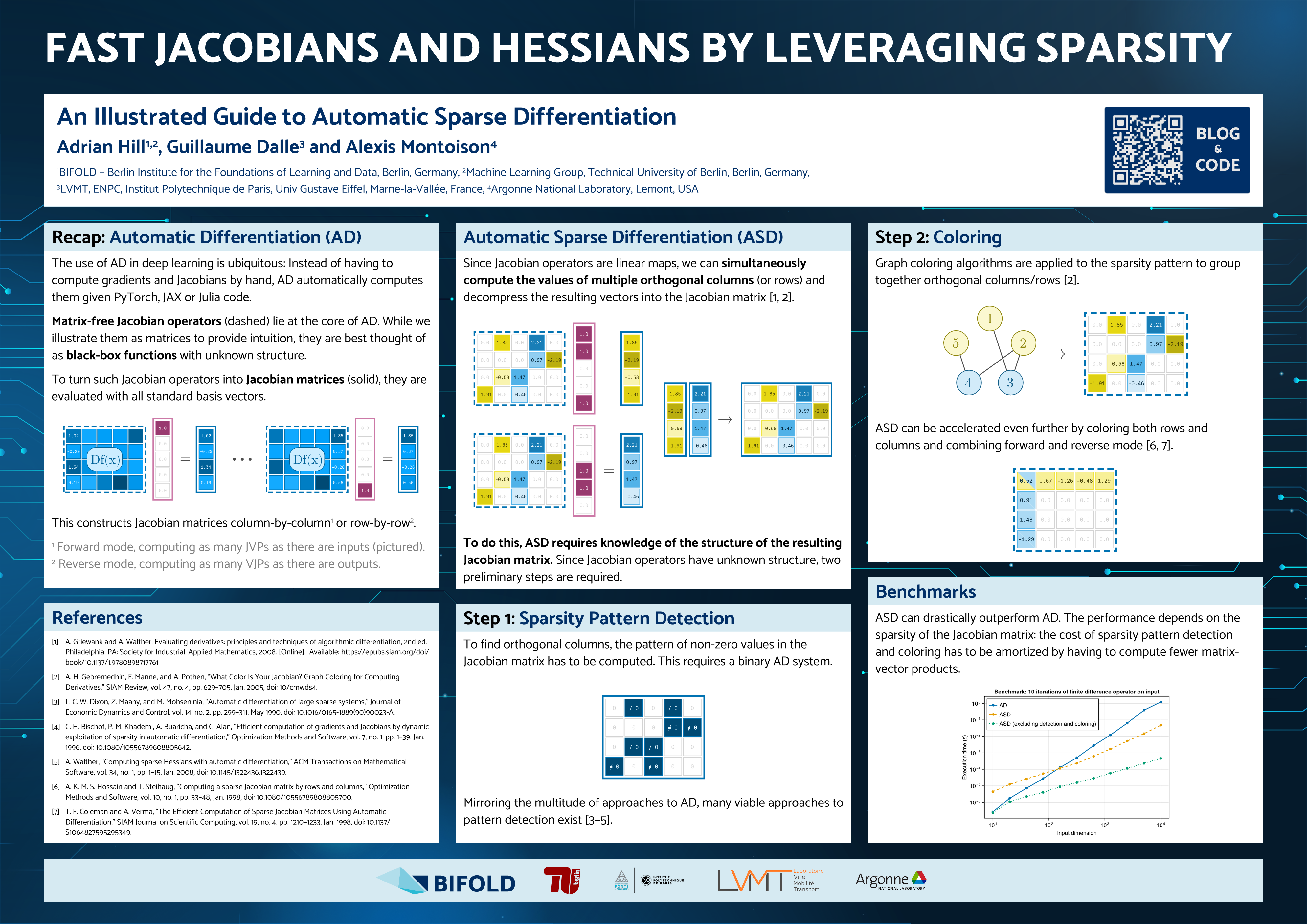
In numerous applications of machine learning, Hessians and Jacobians exhibit sparsity, a property that can be leveraged to vastly accelerate their computation. While the usage of automatic differentiation in machine learning is ubiquitous, automatic sparse differentiation (ASD) remains largely unknown. This post introduces ASD, explaining its key components and their roles in the computation of both sparse Jacobians and Hessians. We conclude with a practical demonstration showcasing the performance benefits of ASD._First-order optimization is ubiquitous in machine learning (ML) but second-order optimization is much less common. The intuitive reason is that high-dimensional vectors (gradients) are cheap, whereas high-dimensional matrices (Hessians) are expensive. Luckily, in numerous applications of ML to science or engineering, Hessians and Jacobians exhibit sparsity: most of their coefficients are known to be zero. Leveraging this sparsity can vastly accelerate automatic differentiation (AD) for Hessians and Jacobians, while decreasing its memory requirements. Yet, while traditional AD is available in many high-level programming languages like Python and Julia, automatic sparse differentiation (ASD) is not as widely used. One reason is that the underlying theory was developed outside of the ML research ecosystem, by people more familiar with low-level programming languages.With this blog post, we aim to shed light on the inner workings of ASD, bridging the gap between the ML and AD communities by presenting well established techniques from the latter field. We start out with a short introduction to traditional AD, covering the computation of Jacobians in both forward and reverse mode. We then dive into the two primary components of ASD: sparsity pattern detection and matrix coloring. Having described the computation of sparse Jacobians, we move on to sparse Hessians.We conclude with a practical demonstration of ASD, providing performance benchmarks and guidance on when to use ASD over AD.